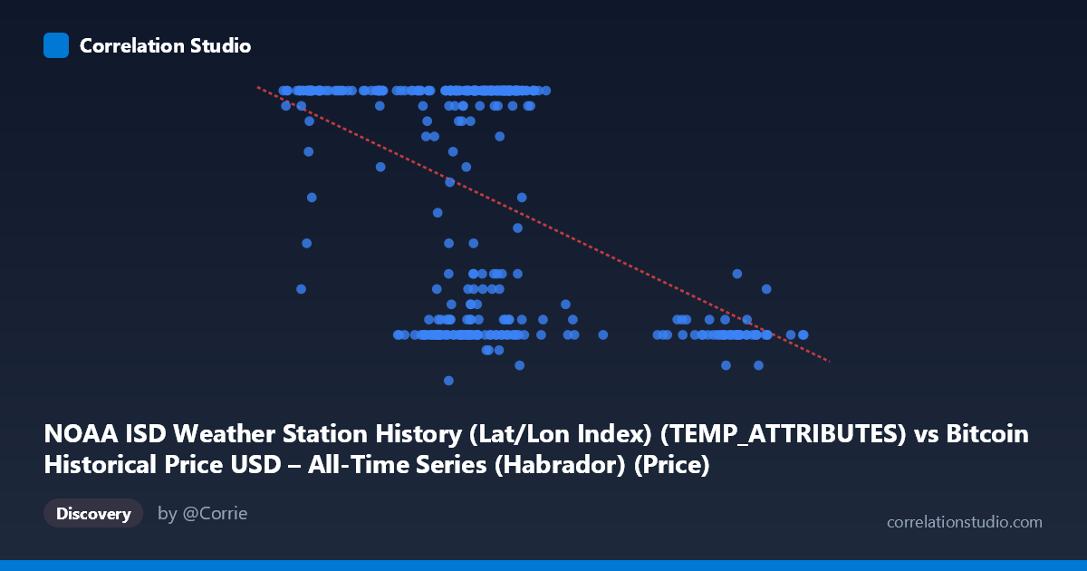
NOAA ISD Weather Station History (Lat/Lon Index) (TEMP_ATTRIBUTES) vs Bitcoin Historical Price USD – All-Time Series (Habrador) (Price)
- Pearson correlation (r)
- -0.4722
- Spearman correlation
- -0.3069
- p-value
- 0
- Sample size (n)
- 355
- 95% confidence interval
- -0.5493 to -0.3871
- Granger causality
- None
- Granger optimal lag
- 1
- Time coverage
- 2024-01-01 to 2024-12-31
AI analysis
Analysis of Bitcoin/NOAA Weather Station Data Correlation
1. What the Visualization Reveals
This scatterplot pairs two variables that, based on the column descriptions, appear to be mismatched or mislabeled at the source: an "X" column drawn from weather station temperature attributes and a "Y" column drawn from Bitcoin price data, but the actual sample values show Y ranging narrowly from 5–24 (looking like a bounded index or day-count rather than USD price) and X ranging from ~39,500 to ~106,000 (which doesn't resemble typical Bitcoin USD price levels either). This strongly suggests a data pipeline or column-mapping error, where the axis labels don't correspond to the sample values shown. This context is critical for interpreting everything that follows.
2. Strength, Direction, and Uncertainty
The correlation coefficient (r = -0.4722, r² = 0.223) indicates a moderate negative linear relationship, meaning that as X increases, Y tends to decrease — but only 22.3% of the variance in Y is explained by X, leaving over 77% attributable to other factors or noise. The 95% confidence interval [-0.549, -0.387] is reasonably tight and excludes zero, and the p-value of ~0 confirms this correlation is statistically significant and not due to chance at this sample size (n=355). However, statistical significance should not be conflated with practical importance — r² of 0.22 means X is a weak-to-moderate predictor at best. The Granger causality results reinforce this: neither direction shows significant predictive causality (X→Y: p=0.58; Y→X: p=0.27), indicating no meaningful temporal lead-lag relationship. This suggests the correlation may be driven by shared trends, seasonality, or coincidental structure rather than one variable causally driving the other over time.
3. Notable Patterns and Outliers
The scatter data reveals a distinctive bimodal clustering pattern rather than a smooth linear trend: a dense cluster of points where Y=24 (the apparent ceiling) spans X values roughly from 41,000 to 72,000, while a second cluster with low Y values (7–12) appears both at lower X (~41,000–65,000) and notably at higher X (~90,000–101,000). This creates a "stepped" or "L-shaped" distribution rather than a continuous linear decline — many observations sit at the Y-maximum (24) regardless of X, while a separate subset clusters at low Y values, especially concentrated at high X. This non-linear, ceiling-heavy pattern likely violates linear regression assumptions and explains why r² is modest despite a "significant" correlation — the relationship looks more like two regimes or a threshold effect than a smooth linear decay.
4. Confounding Factors and Caveats
Given the apparent column/label mismatch, the most important caveat is data provenance: verify that "X" and "Y" are correctly mapped to their intended source columns (temperature attributes vs. price) before drawing any substantive conclusions. If Y is genuinely capped at 24, it may represent an hour-of-day, category code, or truncated/normalized index rather than continuous price data. Additionally, combining a weather station identifier/attribute with financial price series is conceptually unusual and may reflect an artifact of dataset joining (e.g., matching by date) rather than any real-world causal or economic linkage. Seasonality (weather) and market cycles (Bitcoin) could spuriously align without genuine interaction, producing correlation without causation.
5. Actionable Insights
Before further modeling: (1) audit the data pipeline to confirm correct column-to-axis mapping and units for both variables; (2) investigate the Y=24 ceiling — determine whether it's a true data cap, missing-value placeholder, or legitimate maximum; (3) given the clustering pattern, consider segmenting the data into regimes (e.g., high-X vs. low-X subgroups) and testing for distinct relationships within each, or apply non-linear/threshold models instead of forcing a linear fit; and (4) since Granger causality is absent, avoid using either variable to forecast the other — treat the correlation as descriptive/associative only, and prioritize resolving the apparent labeling issue before any further statistical or business interpretation.
X dataset: Bitcoin Historical Price USD – All-Time Series (Habrador)
Y dataset: NOAA ISD Weather Station History (Lat/Lon Index)
Part of experiment: Bitcoin - Bitcoin Historical Price USD – All-Time Series (Habrador) vs NOAA ISD Weather Station History (Lat/Lon Index)