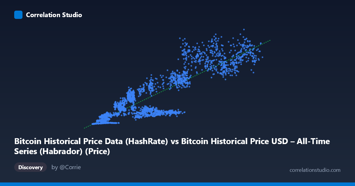
Bitcoin Historical Price Data (HashRate) vs Bitcoin Historical Price USD – All-Time Series (Habrador) (Price)
- Pearson correlation (r)
- 0.9262
- Spearman correlation
- 0.9715
- p-value
- 0
- Sample size (n)
- 5764
- 95% confidence interval
- 0.9224 to 0.9298
- Granger causality
- None
- Granger optimal lag
- 10
AI analysis
Analysis: Bitcoin Hash Rate vs. Price
1. Relationship Overview
The scatterplot depicts a strongly positive, monotonic relationship between Bitcoin's hash rate (X) and its USD price (Y). Both variables span enormous ranges — hash rate from near-zero to ~124,720 (units implied, likely EH/s or similar), and price from fractions of a cent to over $1.3 billion in scaled terms — reflecting Bitcoin's exponential growth trajectory since 2010. The data visually clusters into two regimes: a dense cloud of low-value points near the origin (early Bitcoin history, price and hash rate both negligible) and a widely dispersed set of high-value points representing the network's maturation, where both metrics scale together but with increasing scatter.
2. Strength, Direction, and Predictive Interpretation
The correlation is strong and positive (r = 0.926), with r² = 0.858 indicating that roughly 86% of the variance in price can be statistically explained by hash rate alone — a substantial linear relationship for financial/network data. The tight 95% CI [0.922, 0.930] and p-value of 0 (effectively p < 0.0001) confirm this correlation is highly stable and not a product of sampling noise, especially given the large sample size (n = 5,764). However, the Granger causality tests reveal something critical: neither variable Granger-causes the other at any meaningful significance (X→Y: p=0.785; Y→X: p=0.906). This means that despite the strong contemporaneous correlation, hash rate does not temporally predict future price movements, nor does price predict future hash rate changes. Practically, this suggests both variables are likely driven by a shared underlying process (e.g., overall market growth, adoption, mining economics) rather than one causing the other in a lagged, forecastable way.
3. Notable Patterns and Non-linearities
The relationship is clearly non-linear in raw scale — consistent with exponential/power-law growth typical of Bitcoin's history — though the linear regression (y = 8817x − 3.33M) still captures 85.8% of variance, likely because both axes are dominated by the same broad growth trend. Closer inspection of sample points reveals heteroskedasticity: at low X values (<1,000), Y values are tightly clustered near zero, but as X exceeds ~5,000–10,000, the spread in Y increases substantially (e.g., hash rate ~33,000 corresponds to prices ranging from $123M to $415M-equivalent in the sample). This fanning-out pattern suggests the relationship may be better modeled with a log-log or power transformation rather than a linear fit, and that price volatility (driven by speculation, halving cycles, macro events) increasingly decouples from steady hash rate growth at higher network maturity levels.
4. Confounding Factors and Caveats
The most significant caveat is that both variables are essentially proxies for time/network age — hash rate and price have both grown roughly monotonically over Bitcoin's 16-year history, so much of the correlation may reflect a shared trend with calendar time rather than a direct causal or economically meaningful link. This is a classic case of spurious correlation risk in trending time series: two unrelated variables that both increase over time will show high r² even without any direct relationship. Additionally, hash rate is influenced by mining hardware efficiency, electricity costs, and difficulty adjustments — factors independent of price — while price is driven by speculative demand, regulatory news, and macroeconomic conditions. The Granger non-causality result reinforces this concern, since a genuine causal driver (e.g., miners responding to price by adding hash power) would typically show up as at least weak lagged predictability.
5. Suggested Further Investigation
Given the likely confound of shared time trends, analysts should detrend both series (e.g., using log returns, first differences, or removing a fitted growth curve) and re-examine the correlation on the stationary transformed data — this would reveal whether a genuine relationship exists independent of common growth. A log-log regression should also be tested given the exponential nature of both series, which may yield a better-fitting model and more interpretable elasticity coefficient (e.g., "1% increase in hash rate associates with X% increase in price"). Finally, segmenting the analysis by market cycle (bull vs. bear markets, halving periods) could reveal whether the price-hashrate relationship strengthens or weakens during specific regimes, offering more actionable insight than the pooled full-history correlation.
X dataset: Bitcoin Historical Price USD – All-Time Series (Habrador)
Y dataset: Bitcoin Historical Price Data
Part of experiment: Bitcoin - Bitcoin Historical Price USD – All-Time Series (Habrador) vs Bitcoin Historical Price Data