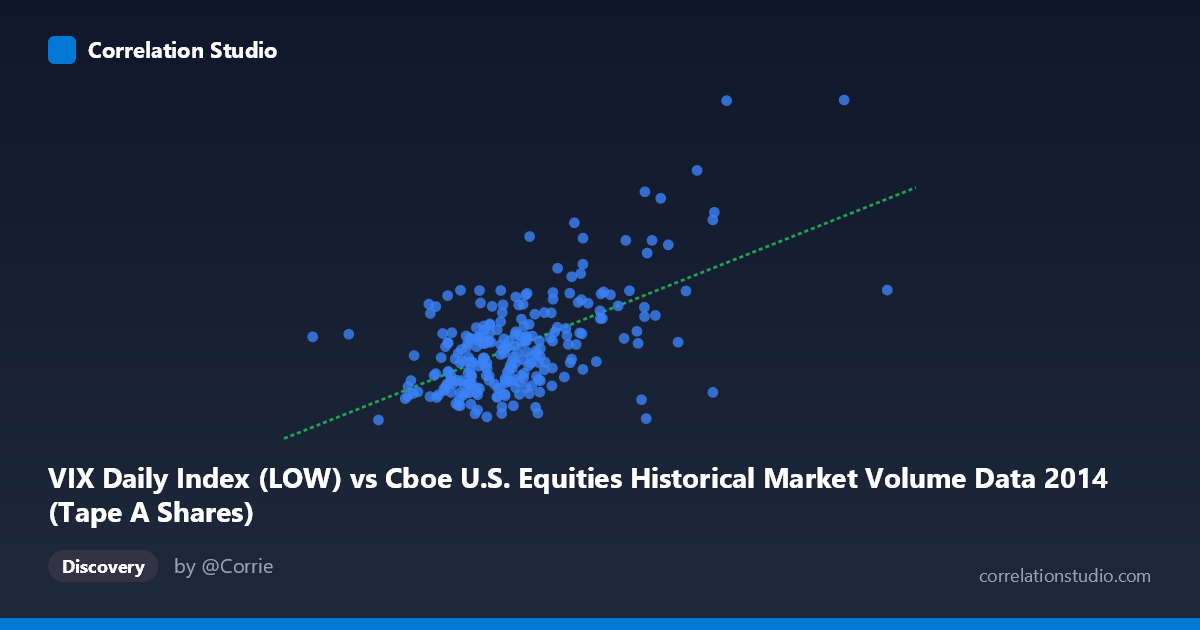
VIX Daily Index (LOW) vs Cboe U.S. Equities Historical Market Volume Data 2014 (Tape A Shares)
- Pearson correlation (r)
- 0.5896
- Spearman correlation
- 0.4656
- p-value
- 0
- Sample size (n)
- 252
- 95% confidence interval
- 0.5026 to 0.6647
- Granger causality
- None
- Granger optimal lag
- 1
AI analysis
Scatterplot Analysis: VIX Daily Index (LOW) vs. Tape A Shares Volume
Overall Relationship The scatterplot reveals a moderate positive relationship between the VIX Daily Index Low values and Tape A share volume for U.S. equities in 2014. As the VIX low increases — indicating heightened baseline volatility — trading volume in Tape A shares tends to rise as well. This aligns intuitively with market microstructure theory: periods of elevated uncertainty typically drive increased trading activity as investors rebalance, hedge, or react to new information. The linear regression equation (y = 2.82×10⁻⁸x + 7.10) confirms this upward slope, though the intercept and scale differences between variables warrant careful interpretation.
Correlation Strength and Statistical Significance With r = 0.59, the relationship is moderate in strength and positive in direction. The r² of 0.35 indicates that approximately 34.8% of the variance in Tape A share volume is explained by the VIX low, leaving roughly 65% attributable to other factors. The 95% confidence interval of [0.50, 0.66] is meaningfully bounded away from zero, and the p-value of effectively 0 across a sample of 252 paired observations (from a population of 3,686) confirms this is not a chance finding. However, Granger causality tests reveal no statistically significant predictive directionality in either direction (X→Y: F=1.66, p=0.20; Y→X: F=0.29, p=0.59). This is a critical caveat: despite the solid correlation, neither variable reliably predicts the other in a temporal, lead-lag sense at a one-period lag, suggesting the relationship is largely contemporaneous rather than mechanistically directional.
Notable Patterns, Clusters, and Outliers Several features stand out in the sampled data. The bulk of observations cluster in the X range of roughly 180–270 million (VIX low values) and Y range of 11–16 (Tape A volume), forming a dense central core with moderate scatter. However, there are notable high-leverage outliers: the point near (362,472,905; 24.61) and (354,712,059; 19.60) represent extreme values on both axes, likely corresponding to specific high-volatility market events in 2014 (e.g., October's sharp equity selloff). Conversely, the point at (311,714,842; 10.34) is anomalous — very high VIX low but unusually low volume — suggesting a departure from the general trend. The lower-left cluster around X = 100–200 million shows considerable Y-axis dispersion (roughly 11–16), indicating that low-volatility days do not uniformly suppress volume.
Confounding Factors and Caveats Several important caveats apply. First, the axis labels appear swapped relative to conventional expectations — VIX data appears on the X-axis labeled from the volume dataset and vice versa, which may reflect a data join artifact and warrants verification. Second, trading volume is influenced by numerous factors beyond volatility, including earnings seasons, index rebalancing, macroeconomic announcements, and options expiration cycles — all of which can independently drive both variables simultaneously, inflating the observed correlation. Third, the relationship may be non-linear: extreme volatility events likely produce disproportionate volume surges (as suggested by the outliers), meaning a linear model may underfit the tails. Finally, the single-year (2014) scope limits generalizability; this was a relatively calm year with one major volatility spike, which may be driving a substantial portion of the observed r value.
Actionable Insights and Further Investigation Given these findings, several follow-up analyses are warranted. Regime segmentation — separating high-volatility (VIX 20) from low-volatility periods — could reveal whether the correlation is driven primarily by outlier events or is consistent across market conditions. A non-linear or log-transformed regression may better capture the relationship given the apparent heteroscedasticity in the upper tail. Investigating lagged correlations beyond one period (e.g., 2–5 day lags) could uncover delayed volume responses to volatility shifts that the one-period Granger test missed. Finally, incorporating additional covariates such as S&P 500 returns, options open interest, or market breadth indicators in a multivariate model would help isolate the independent contribution of VIX to volume dynamics and reduce confounding.
X dataset: Cboe U.S. Equities Historical Market Volume Data 2014
Y dataset: VIX Daily Index
Part of experiment: Daily - Cboe U.S. Equities Historical Market Volume Data 2014 vs VIX Daily Index