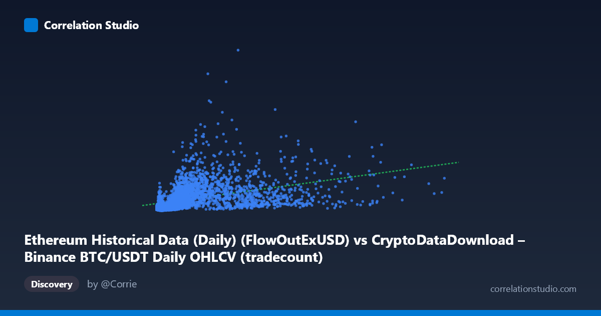
Ethereum Historical Data (Daily) (FlowOutExUSD) vs CryptoDataDownload – Binance BTC/USDT Daily OHLCV (tradecount)
- Pearson correlation (r)
- 0.4118
- Spearman correlation
- 0.7022
- p-value
- 0
- Sample size (n)
- 3191
- 95% confidence interval
- 0.3826 to 0.4402
- Granger causality
- None
- Granger optimal lag
- 10
AI analysis
Analysis of the Ethereum FlowOutExUSD vs. BTC/USDT Tradecount Relationship
1. What the Visualization Reveals
The scatterplot shows a positive but noisy relationship between the two variables, with substantial scatter around the fitted regression line. Most data points cluster in the lower-left region (X < 3,000,000; Y < 1,500,000,000), with a long right-tail of higher X values that are relatively sparse. This right-skewed distribution — evident from the mean (1.97M) sitting well below where the range extends to (15.36M) — indicates the relationship is not uniformly sampled across the X range, and the bulk of the correlation signal is driven by the dense lower-range cluster.
2. Strength, Direction, and Statistical Confidence
The Pearson correlation (r = 0.412) indicates a moderate positive relationship, but r² = 0.170 reveals that only about 17% of the variance in Y is explained by X — meaning roughly 83% of the variability in tradecount is driven by other factors entirely unrelated to this flow metric. The 95% CI [0.383, 0.440] is fairly tight given the large sample size (n=3,191), and the p-value of ~0 confirms this correlation is highly statistically significant — it is very unlikely to be due to chance. However, statistical significance should not be conflated with practical importance: with r² this low, X is a weak standalone predictor of Y. Critically, the Granger causality tests show no significant predictive direction in either direction (X→Y: p=0.78; Y→X: p=0.39), meaning that despite the contemporaneous correlation, neither variable's historical values help forecast the other's future values. This suggests the correlation is likely driven by a shared external factor (e.g., overall market growth/activity trends) rather than one variable causing or leading the other.
3. Notable Patterns and Non-linear Features
The note that Spearman ρ exceeds Pearson r is an important clue: it implies a monotonic but non-linear relationship — likely logarithmic or power-law in shape, which is common when comparing a heavily right-skewed volume/flow metric (X) against a count-based metric (Y). Sample points show considerable heteroscedasticity: at low X values (e.g., X≈2,000–10,000), Y ranges wildly from ~60M to ~980M, while at higher X values (X5M) the spread narrows somewhat. This "funnel" pattern (variance decreasing as X increases) is a classic sign that a log transformation of X (and possibly Y) would produce a better-fitting, more homoscedastic model. There's no obvious clustering into discrete groups, but the extreme right-tail values (X 8M) appear to behave as high-leverage points that could disproportionately influence the linear fit.
4. Confounding Factors and Caveats
Several caveats limit interpretation: (1) Cross-dataset mismatch — X is an Ethereum exchange flow metric while Y is labeled as BTC/USDT tradecount from Binance; these come from different assets/datasets, so any correlation may simply reflect broad crypto-market co-movement (both assets tend to see volume/activity spike together during bull/bear cycles) rather than a direct mechanistic link. (2) Time-trend confounding — both series likely trend upward over 2017–2026 as crypto markets matured and grew, meaning the correlation could substantially be an artifact of shared secular growth (a spurious correlation from non-stationarity) rather than genuine covariation. (3) Outlier sensitivity — given the extreme range of X (2,153 to 15.36M) and Y (13.9M to 7.36B), a small number of extreme observations could be inflating or deflating r and the regression slope.
5. Actionable Insights and Further Investigation
Given the weak r², non-significant Granger causality, and Spearman/Pearson divergence, this correlation should not be used for forecasting or trading signal generation in its current form. Recommended next steps: (1) Apply log-log transformation to both variables and re-fit (linear or polynomial) to test if it substantially improves r² and normalizes residuals. (2) De-trend both series (e.g., using differencing or detrending against time) to test whether the correlation persists after removing shared secular growth — this would clarify whether the relationship is genuine or a trend artifact. (3) Since both series originate from different underlying assets, consider testing whether a shared latent factor (e.g., total crypto market cap, BTC price, or overall trading volume) better explains the covariation. (4) Given non-stationarity is likely, formally test for cointegration rather than relying on simple correlation/Granger tests on levels.
X dataset: CryptoDataDownload – Binance BTC/USDT Daily OHLCV
Y dataset: Ethereum Historical Data (Daily)
Part of experiment: Bitcoin - CryptoDataDownload – Binance BTC/USDT Daily OHLCV vs Ethereum Historical Data (Daily)