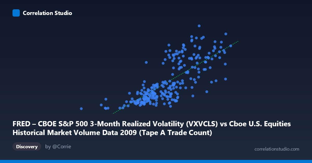
FRED – CBOE S&P 500 3-Month Realized Volatility (VXVCLS) vs Cboe U.S. Equities Historical Market Volume Data 2009 (Tape A Trade Count)
- Pearson correlation (r)
- 0.7559
- Spearman correlation
- 0.7851
- p-value
- 0
- Sample size (n)
- 252
- 95% confidence interval
- 0.6975 to 0.8043
- Granger causality
- None
- Granger optimal lag
- 1
AI analysis
Analysis: CBOE S&P 500 3-Month Realized Volatility vs. Tape A Trade Count (2009)
Relationship Overview The scatterplot reveals a moderately strong positive relationship between CBOE S&P 500 3-month realized volatility (VXVCLS) and Tape A trade counts across U.S. equity exchanges in 2009. As volatility rises, trade counts increase meaningfully, which aligns with well-established market microstructure theory: elevated uncertainty drives higher turnover as market participants rebalance, hedge, and respond to price signals. The linear regression equation (y = 1.549×10⁻⁵x + 7.710) suggests that for every unit increase in trade volume, implied volatility rises by approximately 0.0000155 index points — a small but statistically meaningful slope given the scale of the X variable.
Correlation Strength and Statistical Interpretation The Pearson correlation of r = 0.7559 indicates a robust positive association, with r² = 0.5714 confirming that approximately 57.1% of the variance in 3-month realized volatility is explained by Tape A trade counts. This is a meaningful explanatory share, though it equally means ~43% of volatility variation is driven by factors outside this model. The 95% confidence interval of [0.6975, 0.8043] is relatively tight given the sample of n = 252, and the p-value of essentially zero provides overwhelming evidence against the null hypothesis of no correlation. Critically, however, Granger causality tests find no significant predictive directionality in either direction (X→Y: F = 0.264, p = 0.608; Y→X: F = 0.007, p = 0.934), meaning that while the two variables move together contemporaneously, neither reliably leads or predicts the other at a one-period lag. This is a crucial caveat: correlation here appears to reflect simultaneous co-movement rather than a temporal cause-and-effect chain.
Notable Patterns, Clusters, and Outliers The scatterplot exhibits a few structurally interesting features. There is a dense cluster at lower trade counts (roughly 362,000–1,500,000) paired with lower volatility (22–32), suggesting calm, lower-activity market conditions dominated much of 2009. A second, more dispersed cluster appears at higher trade counts (1,800,000–2,550,000) associated with elevated volatility (38–55), likely corresponding to periods of market stress in early-to-mid 2009 as the financial crisis was resolving. The point (362081, 22.43) stands out as a potential low-volume outlier at the lower-left extreme, while (2549191.92, 47.03) and (2149162.38, 50.43) anchor the upper-right. A subtle non-linearity may be present — the relationship appears to steepen at higher volume levels — suggesting a linear model, while adequate, may not fully capture the dynamics at market extremes.
Confounding Factors and Caveats Several important caveats temper interpretation. First, 2009 was an extraordinary year — spanning the tail of the global financial crisis and a historic market recovery — making any annual relationship potentially unrepresentative of structural norms. Second, Tape A trade counts aggregate multiple exchange venues, and compositional shifts (e.g., HFT activity spikes, dark pool routing changes) could inflate trade counts independently of volatility. Third, the axis labels appear transposed in the dataset descriptions (X is labeled as VXVCLS but the dataset metadata refers to volume, and vice versa), warranting careful verification before acting on directional claims. Fourth, the lack of Granger causality may reflect the one-day lag being too coarse — intraday or higher-frequency analysis might reveal genuine lead-lag structures missed here.
Actionable Insights and Further Investigation Practitioners interested in volatility forecasting or market liquidity modeling should note that while trade activity and realized volatility share substantial co-movement, neither variable reliably predicts the other at daily frequency, limiting their use as standalone leading indicators for one another. Further investigation should include: (1) testing multiple lag lengths in Granger analysis to rule out relationships beyond one period; (2) regime-segmenting the data (e.g., pre/post March 2009 market bottom) to assess whether the correlation is stable or crisis-driven; (3) adding control variables such as bid-ask spreads, VIX levels, or macro news event indicators to isolate the independent effect of trade volume on volatility; and (4) replicating the analysis across multiple years to determine whether the r = 0.76 relationship is structurally persistent or an artifact of the extraordinary 2009 environment.
X dataset: Cboe U.S. Equities Historical Market Volume Data 2009
Y dataset: FRED – CBOE S&P 500 3-Month Realized Volatility
Part of experiment: Daily - Cboe U.S. Equities Historical Market Volume Data 2009 vs FRED – CBOE S&P 500 3-Month Realized Volatility