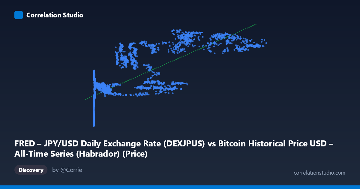
FRED – JPY/USD Daily Exchange Rate (DEXJPUS) vs Bitcoin Historical Price USD – All-Time Series (Habrador) (Price)
- Pearson correlation (r)
- 0.7397
- Spearman correlation
- 0.7702
- p-value
- 0
- Sample size (n)
- 3946
- 95% confidence interval
- 0.7253 to 0.7535
- Granger causality
- None
- Granger optimal lag
- 1
- Time coverage
- 2010-07-19 to 2026-04-28
- Recomputed on refreshed data
- 2026-10-20 (r was 0.7397)
AI analysis
Analysis: Bitcoin Price (X) vs. JPY/USD Exchange Rate (Y)
1. What the visualization reveals
The scatterplot shows a moderately strong positive association between Bitcoin's USD price and the JPY/USD exchange rate (i.e., yen weakness against the dollar). At low Bitcoin prices (under ~$1,000, corresponding to Bitcoin's early years, 2010–2013), the yen trades in the mid-70s to 100 range. As Bitcoin's price climbs into the tens of thousands and beyond, JPY/USD values cluster in the 105–160 range, with the highest yen values (140–160) coinciding with Bitcoin prices above $90,000. The relationship is not a tight line but rather a broad upward-sloping band with considerable vertical scatter at any given X value — for instance, Bitcoin prices near 10,000–17,000 correspond to Y values ranging widely from ~104 to ~140.
2. Strength, direction, and statistical framing
The correlation coefficient (r = 0.74) indicates a strong positive linear relationship, and r² = 0.547 means that roughly 55% of the variance in the JPY/USD rate is statistically associated with Bitcoin's price level — leaving nearly half unexplained by this single variable. The tight 95% CI [0.725, 0.754] and p-value of ~0 confirm this correlation is not a statistical fluke; with nearly 4,000 paired observations, we can be highly confident a real, non-zero association exists. However, statistical significance should not be conflated with causal or practical strength: r² of 0.55 still leaves substantial room for other drivers. Critically, the Granger causality tests show no significant predictive direction in either direction (X→Y: p=0.48; Y→X: p=0.21). This means neither series' past values help forecast the other's future values beyond what each series' own history provides — the correlation is almost certainly driven by both variables trending over a shared timeframe rather than one causing the other.
3. Notable patterns and outliers
The most conspicuous feature is the temporal clustering effect: data points aren't randomly distributed but trace out Bitcoin's boom-bust cycles overlaid on yen depreciation trends. The 2010–2013 period contributes a dense cluster of low-X, low-Y points (Bitcoin <$1,000, yen 75–100). A middle cluster (Bitcoin $5,000–$30,000, yen 105–140) shows the most scatter and non-linearity — including local dips where Bitcoin fell (e.g., $10,000–17,000 range) while yen values were still elevated (130–140), suggesting the two series decoupled during certain sub-periods. At the high end (Bitcoin $90,000), yen values compress into a tighter 142–160 band, hinting at a possible saturation or nonlinear (e.g., logarithmic) relationship rather than strictly linear, especially given Bitcoin's exponential growth scale.
4. Confounding factors and caveats
This is a classic case of spurious correlation risk via shared trend/time confounding. Both Bitcoin's price and JPY/USD have exhibited long-term secular trends over the 2010–2026 window (Bitcoin appreciating enormously; yen weakening due to Bank of Japan policy, US-Japan rate differentials, etc.) that are unrelated to each other in mechanism. Any two upward-trending time series will show inflated correlation purely from co-trending, and the lack of Granger causality strongly supports this interpretation — there's no evidence of a real predictive or mechanistic link. Additional caveats: Bitcoin's X range spans over 6 orders of magnitude (0.05 to 124,720), so linear regression is heavily influenced by extreme high-end values; the data likely isn't stationary (both series have unit-root-like trending behavior), which itself can produce misleading correlation/regression statistics; and macro confounders (global risk sentiment, USD strength broadly, interest rate cycles, quantitative easing policies) could simultaneously affect both series independently.
5. Actionable insights
Given the trend-confounding risk, analysts should test correlation on detrended or differenced data (e.g., daily/weekly returns rather than price levels) to check if the relationship holds once shared trends are removed — this often eliminates spurious correlations in trending financial series. A cointegration test (e.g., Engle-Granger or Johansen) would clarify whether these two series share a long-run equilibrium relationship despite the lack of Granger causality in levels. Additionally, segmenting the analysis by discrete Bitcoin market cycles (2010–2013, 2017 bubble, 2020–2021 bull run, 2024–2026) would reveal whether the relationship is consistent or regime-dependent. Given the non-Granger-causal result, this pairing should not be used for predictive trading signals in either direction; instead, treat it as a descriptive historical co-movement likely reflecting broader global macro conditions (dollar strength, risk-on/risk-off cycles) rather than a direct economic linkage between Bitcoin and Japanese currency markets.
X dataset: Bitcoin Historical Price USD – All-Time Series (Habrador)
Y dataset: FRED – JPY/USD Daily Exchange Rate
Part of experiment: Bitcoin - Bitcoin Historical Price USD – All-Time Series (Habrador) vs FRED – JPY/USD Daily Exchange Rate