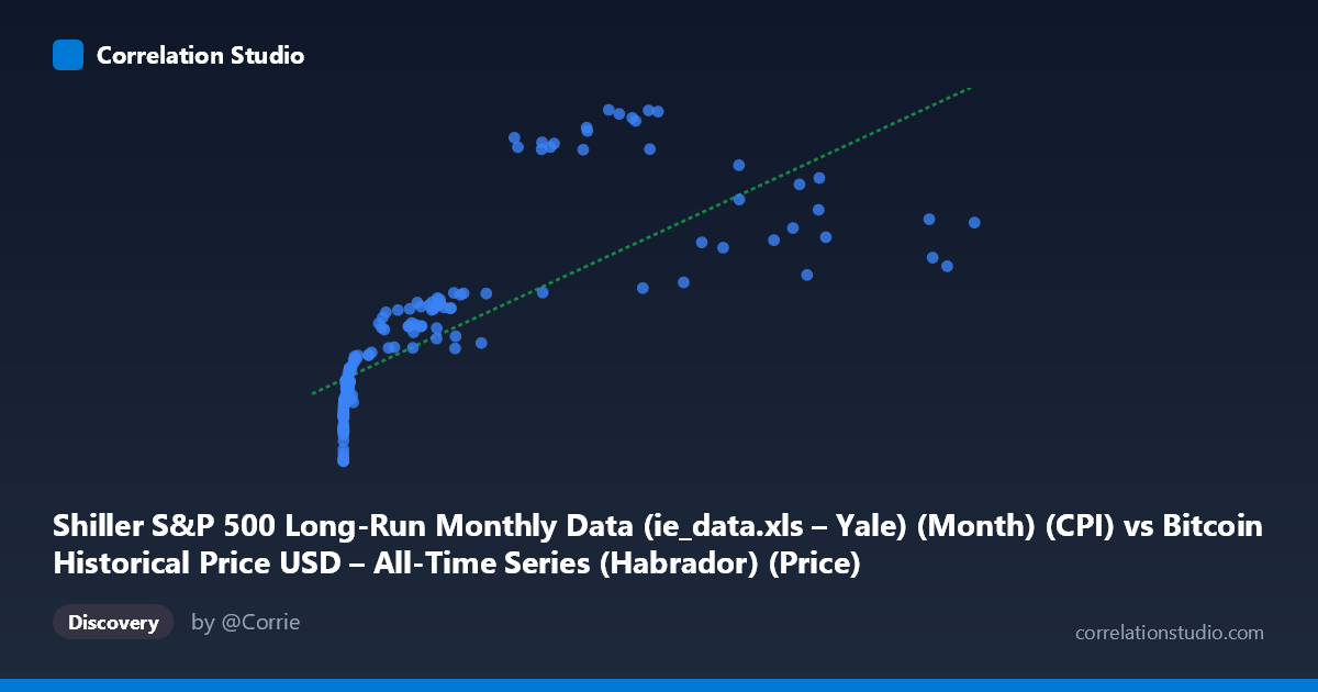
Shiller S&P 500 Long-Run Monthly Data (ie_data.xls – Yale) (Month) (CPI) vs Bitcoin Historical Price USD – All-Time Series (Habrador) (Price)
- Pearson correlation (r)
- 0.7662
- Spearman correlation
- 0.9635
- p-value
- 0
- Sample size (n)
- 158
- 95% confidence interval
- 0.693 to 0.8238
- Granger causality
- Y → X
- Granger optimal lag
- 1
AI analysis
Analysis: Bitcoin Price vs. CPI-Adjusted S&P 500 Data
1. What the Visualization Reveals
The scatterplot shows a positive but non-linear relationship between two variables that are, on their face, mismatched in scale and nature: Bitcoin's USD price (ranging from fractions of a cent to over $61,000) plotted against a Shiller CPI series (ranging narrowly between 218–306). The data points cluster heavily at low X-values (under ~15,000) with a long right tail extending to Bitcoin's all-time-high price range. This clustering pattern — dense at low X, sparse but rising at high X — is characteristic of two time series that both trend upward over a shared calendar period rather than variables with a direct causal or mechanical link.
2. Strength, Direction, and Uncertainty
The Pearson correlation (r = 0.766, r² = 0.587) indicates a strong positive linear association, with the linear model explaining 58.7% of the variance in Y. The 95% CI [0.693, 0.824] is reasonably tight and excludes zero, and the p-value ≈ 0 confirms this correlation is highly unlikely to be due to chance in this sample. However, r² leaves ~41% of variance unexplained, meaning a single linear fit is a mediocre predictor of CPI from Bitcoin price alone. The Granger causality results are notable and counterintuitive: they suggest Y (CPI) Granger-causes X (Bitcoin price) at 1 lag (F=4.13, p=0.044), while Bitcoin price does not Granger-cause CPI (p=0.559). Practically, this means past CPI values have some statistically detectable predictive power for future Bitcoin prices, but not vice versa — though this is likely an artifact of shared trends rather than genuine economic causation (see caveats below).
3. Notable Patterns and Non-linear Features
The data show clear curvature: Y rises quickly at low X, then the rate of increase in Y slows even as X grows by orders of magnitude (e.g., X moves from ~10,000 to ~46,000 while Y only shifts from ~257 to ~280–290). This concave, saturating shape — consistent with the note that Spearman ρ exceeds Pearson r — suggests a logarithmic or power relationship (Y ~ log(X)) would fit better than the linear model. There's also visible scatter/noise at similar X values yielding different Y (e.g., X≈28,000–30,000 produces Y from 296 to 305), indicating additional unmodeled variability, likely tied to specific time periods rather than X itself.
4. Confounding Factors and Caveats
The most important caveat: this is very likely a spurious correlation driven by mutual time trends, not a genuine economic relationship. Bitcoin price and CPI-adjusted Shiller data both trended upward over 2010–2023 due to unrelated macro forces (Bitcoin adoption/speculation cycles vs. long-run inflation and equity market growth). Neither variable plausibly causes the other in a real-world mechanistic sense; the "Y Granger-causes X" finding almost certainly reflects shared trend/autocorrelation structure rather than CPI driving Bitcoin markets. Additional concerns: extreme X skew (mean 9,535 vs. median likely much lower, with a max of 61,374) means a few high-X points exert outsized leverage on the linear fit; the pairing methodology (aligning a monthly Shiller series with a Bitcoin price series that likely didn't exist pre-2009) may introduce artificial date-matching artifacts; and both series exhibit strong internal autocorrelation, which inflates apparent correlation and invalidates standard significance assumptions (the p≈0 should be treated cautiously).
5. Suggestions for Further Investigation
To draw more meaningful conclusions: (1) fit and compare a log-linear or polynomial model (Y ~ log(X)) given the evident curvature and Spearman/Pearson discrepancy; (2) detrend or difference both series (e.g., use returns/growth rates instead of levels) before testing correlation and Granger causality, since levels of trending series routinely produce misleading relationships; (3) explicitly test for and control autocorrelation/unit roots (e.g., Augmented Dickey-Fuller test, cointegration analysis) before trusting Granger causality results; and (4) consider whether a third variable (e.g., overall market liquidity, USD inflation, or risk-on sentiment) is a common driver of both series, which would better explain the observed association than any direct link between Bitcoin price and this CPI-adjusted metric.
X dataset: Bitcoin Historical Price USD – All-Time Series (Habrador)
Y dataset: Shiller S&P 500 Long-Run Monthly Data (ie_data.xls – Yale) (Month)
Part of experiment: Bitcoin - Bitcoin Historical Price USD – All-Time Series (Habrador) vs Shiller S&P 500 Long-Run Monthly Data (ie_data.xls – Yale) (Month)