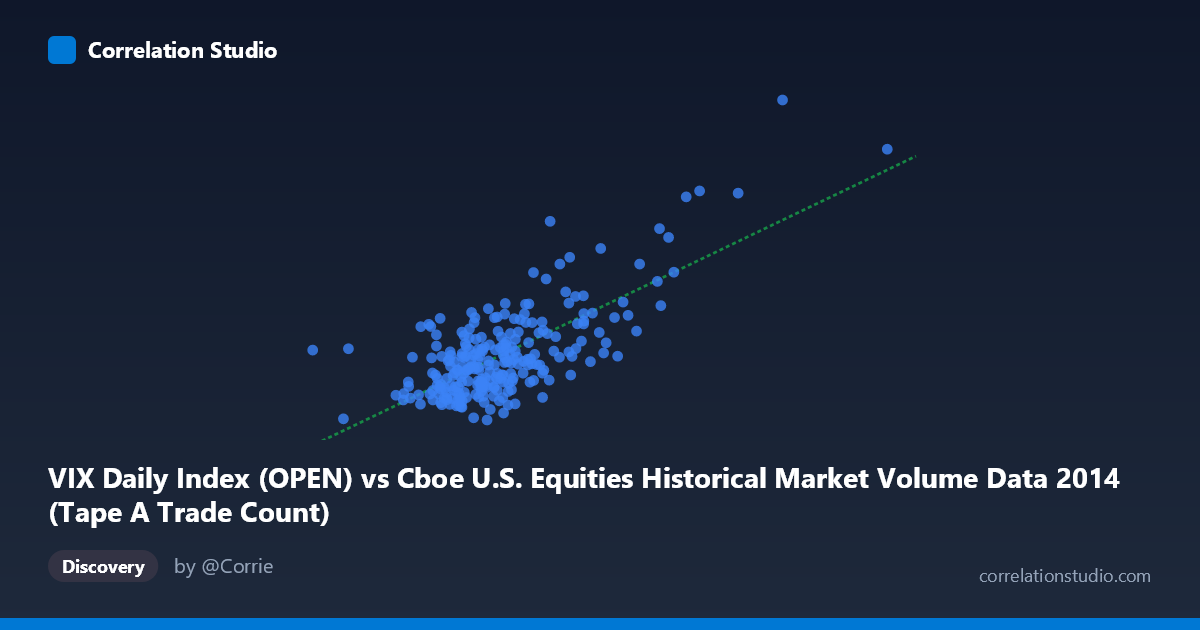
VIX Daily Index (OPEN) vs Cboe U.S. Equities Historical Market Volume Data 2014 (Tape A Trade Count)
- Pearson correlation (r)
- 0.7201
- Spearman correlation
- 0.5414
- p-value
- 0
- Sample size (n)
- 252
- 95% confidence interval
- 0.6548 to 0.7747
- Granger causality
- None
- Granger optimal lag
- 1
AI analysis
Scatterplot Analysis: VIX Open vs. Tape A Trade Count (2014)
Relationship Overview The scatterplot reveals a moderately strong positive relationship between the Cboe VIX Daily Index (Open) and Tape A Trade Count across U.S. equities exchanges in 2014. As VIX open values increase — indicating rising market volatility expectations — trade counts on Tape A tend to rise correspondingly. This is intuitively coherent: periods of elevated volatility typically drive heightened trading activity as market participants react to uncertainty, reposition portfolios, or execute hedging strategies. The linear regression equation (y = 8.07×10⁻⁶x + 4.648) confirms a positive slope, though the relatively small coefficient reflects the scale disparity between the two variables.
Correlation Strength and Statistical Significance The Pearson correlation of r = 0.72 indicates a moderately strong positive association, with r² = 0.5185 meaning that approximately 51.9% of the variance in Tape A Trade Count is explained by VIX Open values — a meaningful but incomplete explanation. Nearly half the variance remains attributable to other factors. The 95% confidence interval of [0.655, 0.775] is relatively tight and sits well above zero, reinforcing reliability of the estimate. With a p-value effectively equal to zero across a paired sample of n = 252 (drawn from a population of N = 3,686), the correlation is statistically unambiguous. However, the Granger causality analysis reveals no significant temporal predictive relationship in either direction — X→Y (F = 3.15, p = 0.077) narrowly misses the conventional 0.05 threshold, and Y→X (F = 0.54, p = 0.46) is clearly non-significant. This means that while the two variables move together, past VIX values do not reliably predict future trade counts at lag-1, urging caution about inferring any directional or causal mechanism.
Notable Patterns, Clusters, and Outliers The sample points reveal a notable cluster of observations concentrated in the X range of roughly 900,000–1,400,000 and Y range of approximately 11–17, representing the bulk of typical trading days in 2014. Within this core cluster, the relationship appears somewhat diffuse, suggesting considerable day-to-day noise at moderate volatility levels. However, several high-leverage outliers are immediately apparent at the upper end — most notably the point near (2,171,498, 29.26) and another near (1,834,381, 23.55) — which correspond to days of extreme market stress. These high-VIX, high-trade-count observations likely exert disproportionate influence on the regression slope and correlation coefficient. There also appears to be a degree of heteroscedasticity: variance in trade counts widens as VIX values increase, suggesting the linear model's fit is stronger in calm periods than in volatile ones.
Confounding Factors and Interpretive Caveats Several important caveats apply. First, reverse causality is plausible — surges in trade volume themselves can amplify intraday price swings and contribute to elevated VIX readings, making the directional story murky. Second, common drivers such as macroeconomic announcements, Federal Reserve communications, or geopolitical events in 2014 (e.g., Ukraine crisis, oil price collapse) could simultaneously spike both VIX and trading activity, producing correlation without a direct link between the two. Third, the outliers at extreme VIX values may represent a qualitatively different regime (crisis vs. normal) rather than a continuous linear relationship, which would violate a core assumption of the regression model. Fourth, the dataset covers only a single calendar year, limiting generalizability; structural relationships between volatility and volume can shift substantially across different market regimes or years.
Actionable Insights and Further Investigation Practitioners and researchers should consider several follow-up steps. Regime segmentation — splitting the data into low, medium, and high VIX terciles — could reveal whether the relationship is driven almost entirely by tail events. A non-linear model (e.g., log-log regression or spline fit) may capture the apparent heteroscedasticity more effectively than the current linear specification. Given that Granger causality narrowly missed significance at the conventional threshold (p = 0.077 for X→Y), testing longer lag structures or using higher-frequency intraday data could clarify whether a predictive signal exists that a lag-1 daily test cannot resolve. Finally, incorporating additional variables — such as S&P 500 returns, bid-ask spreads, or options market activity — into a multivariate framework would help disentangle the ~48% of unexplained variance and better isolate the true marginal contribution of VIX to trade volume dynamics.
X dataset: Cboe U.S. Equities Historical Market Volume Data 2014
Y dataset: VIX Daily Index
Part of experiment: Daily - Cboe U.S. Equities Historical Market Volume Data 2014 vs VIX Daily Index