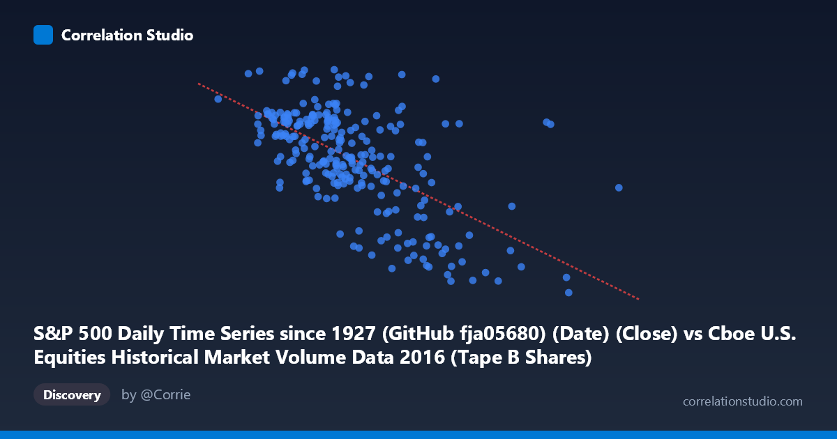
S&P 500 Daily Time Series since 1927 (GitHub fja05680) (Date) (Close) vs Cboe U.S. Equities Historical Market Volume Data 2016 (Tape B Shares)

Pearson correlation (r): -0.6107
Spearman correlation: -0.5802
p-value: 0
Sample size (n): 252
95% confidence interval: -0.6827 to -0.5269
Granger causality: None
Granger optimal lag: 1

AI analysis

Scatterplot Analysis: S&P 500 Close Price vs. Cboe Tape B Share Volume (2016)

Relationship Overview The scatterplot reveals a negative relationship between S&P 500 closing prices (X-axis) and Cboe Tape B share volumes (Y-axis) across 252 trading days in 2016. As the S&P 500 index level rises, Tape B share volume tends to decline, and conversely, lower index levels are associated with higher trading volumes. This inverse pattern is consistent with a well-known market dynamic: elevated uncertainty or market stress — typically associated with lower or falling prices — tends to drive increased trading activity, while calmer, rising markets often see reduced volume participation.

Correlation Strength and Statistical Significance The Pearson correlation of r = −0.611 indicates a moderate-to-strong negative linear association. The coefficient of determination r² = 0.373 means that approximately 37.3% of the variance in Tape B share volume is explained by the S&P 500 closing price level — meaningful, but leaving roughly 63% of volume variation attributable to other factors. The 95% confidence interval of [−0.683, −0.527] is entirely negative and reasonably tight, confirming the direction is reliable. The p-value of essentially zero provides strong evidence against the null hypothesis of no correlation. However, the Granger causality results are notably insignificant in both directions (X→Y: F = 0.517, p = 0.473; Y→X: F = 0.649, p = 0.421), meaning neither variable meaningfully predicts the other's next-day movement at a one-period lag. This is a critical caveat: while a contemporaneous correlation exists, there is no evidence of temporal predictive directionality, suggesting the relationship is coincident rather than leading/lagging.

Notable Patterns and Outliers Several features stand out in the sample data. There is a visible cluster of points in the X range of ~75M–115M (close prices) paired with Y values between roughly 2050–2200, forming the dense core of the distribution. A handful of notable outliers appear at higher X values — points around 170M and 143M show unusually low Y values (~1869–1883), suggesting periods of high index levels coinciding with very low Tape B volume. Conversely, the point near (78.9M, 2265) represents a high-volume, low-price outlier. The linear regression line (y = −2.05×10⁻⁶x + 2313.93) captures the general trend, but the scatter around it is substantial, consistent with the 37% explained variance. There may also be a slight non-linear or heteroscedastic pattern, with variance in Y appearing larger at lower X values.

Confounding Factors and Caveats Several confounds warrant caution. Seasonal effects are likely — trading volumes in 2016 were influenced by calendar patterns (January volatility, summer lulls, year-end repositioning) that independently affect both variables. The 2016 U.S. election and Brexit aftermath created specific volatility episodes that could distort the general relationship. Additionally, Tape B specifically covers NYSE American (AMEX) and regional exchange stocks, which may respond differently to broad market conditions than the S&P 500 large-cap index captures. The axes are also somewhat mismatched conceptually — S&P 500 price level versus share count volume rather than dollar-volume or volatility — meaning the correlation partly reflects a long-term price trend against volume trends rather than a purely dynamic relationship. The absence of Granger causality at lag-1 also suggests the correlation may be driven by shared exposure to a third factor, such as market volatility (VIX) or macroeconomic regime.

Actionable Insights and Further Investigation Practitioners should avoid interpreting this correlation as predictive at a daily horizon, given the failed Granger tests. Instead, this relationship may be more useful as a regime indicator — persistently low index levels combined with high Tape B volume could signal market stress worth monitoring. For deeper investigation, it would be valuable to: (1) introduce VIX or realized volatility as a covariate to test whether it explains the correlation as a mediator; (2) extend the analysis to multiple years to test whether the 2016 relationship is stable or idiosyncratic; (3) test non-linear models (e.g., polynomial or spline regression) given the visible scatter heterogeneity; and (4) examine dollar-volume or turnover rather than raw share counts, which may provide a more economically meaningful comparison to the price-level index.

X dataset: Cboe U.S. Equities Historical Market Volume Data 2016

Y dataset: S&P 500 Daily Time Series since 1927 (GitHub fja05680) (Date)

Part of experiment: Daily - Cboe U.S. Equities Historical Market Volume Data 2016 vs S&P 500 Daily Time Series since 1927 (GitHub fja05680) (Date)