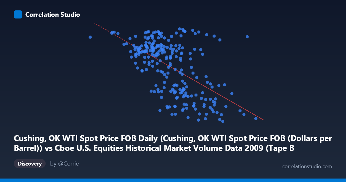
Cushing, OK WTI Spot Price FOB Daily (Cushing, OK WTI Spot Price FOB (Dollars per Barrel)) vs Cboe U.S. Equities Historical Market Volume Data 2009 (Tape B Notional)
- Pearson correlation (r)
- -0.5771
- Spearman correlation
- -0.5243
- p-value
- 0
- Sample size (n)
- 252
- 95% confidence interval
- -0.654 to -0.4883
- Granger causality
- None
- Granger optimal lag
- 1
AI analysis
Scatterplot Analysis: WTI Crude Oil Prices vs. Cboe Tape B Notional Volume (2009)
Relationship Overview
The scatterplot reveals a moderate negative relationship between WTI crude oil spot prices (X-axis) and Cboe Tape B notional trading volume (Y-axis) across 252 trading days in 2009. As oil prices increase, Tape B notional volume tends to decline, and vice versa. This inverse pattern is visually apparent in the spread of points, with higher-volume observations clustering toward lower price levels and lower-volume readings appearing more frequently when oil prices are elevated. The linear regression equation (y = -5.90×10⁻⁹x + 93.07) reflects this downward slope, though considerable scatter around the regression line signals that the relationship is real but far from deterministic.
Correlation Strength and Statistical Significance
The Pearson correlation of r = -0.5771 indicates a moderate negative association. However, r² = 0.333 tells the more practically important story: only 33.3% of the variance in Tape B notional volume is explained by WTI prices, meaning roughly two-thirds of the variation in trading volume is driven by factors entirely unrelated to oil price levels. The 95% confidence interval of [-0.654, -0.488] is meaningfully tight and does not cross zero, and the p-value of effectively zero confirms this relationship is highly unlikely to be a statistical artifact given n = 252 paired observations drawn from a population of N = 3,232. That said, the Granger causality results inject an important caveat: neither variable significantly predicts the other in a temporal sense at the optimal lag of 1 period. X→Y yields F = 0.457 (p = 0.500) and Y→X yields F = 3.462 (p = 0.064) — the latter approaches but does not cross conventional significance thresholds. This means the contemporaneous correlation, while real, does not imply that oil prices lead or predict trading volume (or vice versa) in a directional, causal framework.
Notable Patterns, Clusters, and Outliers
Several structural features are visible in the sample points. There is a notable cluster of high-volume observations (Y ≈ 70–81) concentrated in the mid-to-lower price range (roughly $3.3B–$5.0B), consistent with the negative trend. Conversely, lower-volume readings (Y ≈ 37–52) appear more broadly distributed across higher price levels ($5.5B–$8.7B). A handful of points appear as potential outliers — for instance, the observation at approximately (1.32B, 76.83) sits well to the left of the main cluster, likely representing an early January 2009 session when oil prices were near their post-crisis lows. Similarly, (8.73B, 39.35) anchors the high-price, low-volume extreme. The scatter also hints at possible non-linearity: the negative relationship may steepen at moderate price levels and flatten at extremes, suggesting a simple linear model may not fully capture the true functional form.
Confounding Factors and Interpretive Caveats
Several important caveats apply before drawing conclusions. 2009 was an extraordinary year — it encompassed the tail end of the 2008 financial crisis, a dramatic oil price recovery from ~$35/barrel to ~$80/barrel, and peak post-crisis equity market volatility. These macroeconomic forces almost certainly act as common drivers of both variables independently: risk aversion reduced equity trading volumes while simultaneously suppressing oil prices in early 2009, and subsequent risk appetite recovery elevated both markets, but potentially at different rates across different exchange tapes. Tape B specifically covers NYSE American (AMEX) and regional exchange listings, which may have different sensitivity profiles to macro conditions than Tape A (NYSE) or Tape C (Nasdaq) stocks. Furthermore, the axes appear to show raw notional values and spot prices — without normalizing for concurrent volatility regimes (VIX), broader market volume trends, or seasonal effects — the observed correlation may be partly spurious, a reflection of shared macro timing rather than a direct oil-equity linkage.
Actionable Insights and Further Investigation
Given the moderate but incomplete explanatory power and the absence of Granger causality, practitioners should treat this relationship as contextually informative rather than predictively actionable. Several avenues warrant deeper exploration: (1) Segment the data by market regime (e.g., pre- and post-March 2009 market bottom) to test whether the correlation is stronger in crisis versus recovery phases; (2) Include VIX or credit spread controls to partial out shared macro variance and isolate any residual oil-volume relationship; (3) Compare Tape A and Tape C notional volumes against the same oil price series to determine whether the negative relationship is specific to Tape B listings or a broad equity market phenomenon; (4) Test non-linear specifications (e.g., quadratic or spline regression) given the visual hints of curvature; and (5) Extend the analysis across multiple years to determine whether 2009's unique macro environment is driving this result or whether it reflects a durable structural relationship between energy prices and equity market activity.
X dataset: Cboe U.S. Equities Historical Market Volume Data 2009
Y dataset: Cushing, OK WTI Spot Price FOB Daily
Part of experiment: Daily - Cboe U.S. Equities Historical Market Volume Data 2009 vs Cushing, OK WTI Spot Price FOB Daily