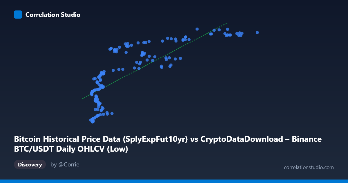
Bitcoin Historical Price Data (SplyExpFut10yr) vs CryptoDataDownload – Binance BTC/USDT Daily OHLCV (Low)
- Pearson correlation (r)
- 0.8018
- Spearman correlation
- 0.833
- p-value
- 0
- Sample size (n)
- 180
- 95% confidence interval
- 0.7426 to 0.8486
- Granger causality
- None
- Granger optimal lag
- 10
- Time coverage
- 2017-08-20 to 2026-02-02
AI analysis
Scatterplot Analysis: SplyExpFut10yr vs. BTC/USDT Daily Low
1. Relationship Overview
The scatterplot shows a positive, moderately strong monotonic relationship between the X variable (a Bitcoin supply-based futures metric) and Y (BTC/USDT daily low price). As X increases from roughly 2,800 to over 115,000, Y rises from approximately $20.2M to $20.8M — note the unusual scale on Y (millions), which suggests this may represent a cumulative or aggregated price series rather than raw daily price. The data does not form a straight line but rather a curved, saturating pattern: Y rises steeply at low X values, then flattens into a plateau above X≈40,000, where most points cluster tightly between Y=20,650,000 and 20,800,000 despite X ranging widely from 40,000 to 115,000.
2. Strength, Direction, and Statistical Confidence
The correlation coefficient (r = 0.80, R² = 0.64) indicates a strong linear association, with 64% of the variance in Y statistically explained by X. However, the 95% CI [0.74, 0.85] is reasonably tight and the p-value is effectively zero, confirming this correlation is highly unlikely to be due to chance in this sample. That said, statistical significance ≠ causal or predictive utility — the Granger causality tests show no significant predictive direction in either direction (X→Y: p=0.44; Y→X: p=0.68). This means that despite the strong contemporaneous correlation, past values of one variable do not reliably help forecast future values of the other at the tested lag structure (10 periods). Practically, this suggests both series may be driven by a common underlying trend (e.g., overall Bitcoin market growth) rather than one causing the other.
3. Notable Patterns and Non-linear Features
The most striking feature is the logarithmic/saturating shape: rapid Y growth for X < 20,000, a transitional zone between 20,000–40,000, and a clear plateau for X 40,000. This directly contradicts the linear regression assumption (y = 5.16x + 2.04E7), which would predict continued proportional growth — the actual data shows diminishing returns. This nonlinearity means the linear R²=0.64 likely understates the true explanatory power available from a log or power-law fit, since much of the unexplained variance comes from forcing a straight line through a curved relationship. There's also a visible cluster of points around X=90,000–105,000 where Y compresses to a narrow band (~20,785,000–20,800,000), suggesting a ceiling effect or market saturation at high supply-metric values.
4. Confounding Factors and Caveats
Both variables are derived from the same underlying asset (BTC) and time period, so they share obvious temporal/trend confounding — as Bitcoin's market matured (2017–2026), both metrics likely increased together due to macro adoption trends, not because either causally drives the other. Additionally, since X is a "supply expectation futures" derivative measure and Y is a spot daily low, both may be jointly influenced by unmodeled factors like market cycles, regulatory news, or halving events. The dataset also isn't a random sample — it's a time series (n=180 sampled from N=3,212), meaning autocorrelation within each variable violates the independence assumption underlying the r/p-value calculations, likely inflating apparent significance.
5. Recommendations for Further Investigation
1. Fit a nonlinear model (logarithmic, power, or piecewise) to capture the plateau pattern more accurately than the linear fit. 2. Test stationarity and detrend both series (e.g., first-differencing) before rerunning correlation and Granger tests, since raw trending series can produce spurious correlations. 3. Investigate the plateau region (X 40,000) separately — is this a genuine ceiling, or an artifact of how "SplyExpFut10yr" is calculated/capped? 4. Given the lack of Granger causality, avoid using this X variable as a predictive leading indicator for Y in trading strategies; treat the relationship as descriptive/contemporaneous only.
X dataset: CryptoDataDownload – Binance BTC/USDT Daily OHLCV
Y dataset: Bitcoin Historical Price Data
Part of experiment: Bitcoin - CryptoDataDownload – Binance BTC/USDT Daily OHLCV vs Bitcoin Historical Price Data