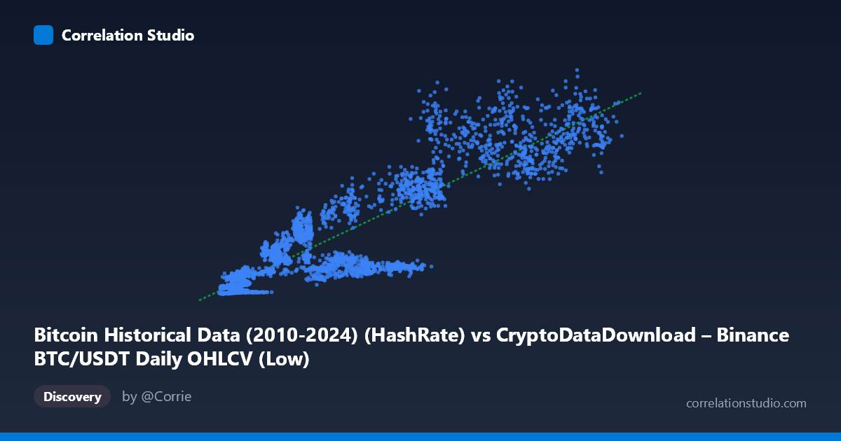
Bitcoin Historical Data (2010-2024) (HashRate) vs CryptoDataDownload – Binance BTC/USDT Daily OHLCV (Low)
- Pearson correlation (r)
- 0.8933
- Spearman correlation
- 0.8842
- p-value
- 0
- Sample size (n)
- 3191
- 95% confidence interval
- 0.8861 to 0.9001
- Granger causality
- None
- Granger optimal lag
- 10
AI analysis
Analysis: Bitcoin Hash Rate vs. Price (Low)
1. Overview of the Relationship
The scatterplot depicts a strong positive association between Bitcoin's hash rate (X) and its daily low price (Y) across 3,191 paired observations spanning 2017–2026. As hash rate increases from roughly 2,800 to 123,000 (units), the corresponding price low rises from single-digit millions to over 1.3 billion, though the sample data suggests these Y-values may represent a scaled or cumulative price metric rather than raw daily lows. The overall shape is a clear upward trend, but it is not perfectly linear — the relationship appears to steepen at higher hash rate values, suggesting a convex or power-law-like curve rather than a strict straight line.
2. Strength, Direction, and Statistical Confidence
The Pearson correlation of r = 0.893 indicates a strong positive linear relationship, with r² = 0.798 meaning nearly 80% of the variance in Y is statistically explained by X under a linear model. The 95% confidence interval [0.886, 0.900] is tight, reflecting the large sample size (n=3,191) and giving high confidence that the true population correlation sits solidly in the "strong" range. The p-value of ~0 confirms this correlation is highly unlikely to be due to chance.
However, the Granger causality results are critical for interpretation: neither direction shows significant predictive causality (X→Y: p=0.49; Y→X: p=0.19) at the optimal lag of 10 periods. This means that despite the strong contemporaneous correlation, hash rate does not temporally predict future price movements, nor does price predict future hash rate in a Granger sense. Practically, this suggests both variables may be driven by a common underlying factor (e.g., overall market cycle, adoption trends, or time itself) rather than one causing the other — the correlation is likely a case of co-trending rather than direct causal linkage.
3. Notable Patterns and Non-Linearity
Examining the sample points reveals a non-uniform, fan-shaped spread: at low hash rates (X < 15,000), Y values are tightly clustered and small (millions), but at high hash rates (X 60,000), Y values scatter widely — some points reach ~1.1 billion while others with similar X sit near 500–600 million. This heteroscedasticity (increasing variance with X) suggests the linear model underfits at the upper range and that a log-log or power transformation might fit better. Additionally, the linear regression's negative intercept (−4.2M) is not economically meaningful (hash rate near zero shouldn't imply negative price), a common artifact when forcing a linear fit to what is likely an exponential growth relationship — consistent with Bitcoin's historical price/hash rate co-evolution.
4. Confounding Factors and Caveats
Both variables are strongly time-trending — hash rate has grown near-monotonically with mining hardware improvements, while price has followed multi-year bull/bear cycles. This shared trend with time is a classic confounder: time itself may be driving both series, inflating the correlation without implying direct mechanistic causality. Other lurking variables include overall crypto market sentiment, halving events, institutional adoption, and macroeconomic liquidity conditions — all of which could simultaneously affect both mining investment (hash rate) and price. The Y-axis column description also raises a data-quality flag: it references "Low" price but the metadata mismatch (mixing hash rate from one dataset with price from another under ambiguous column labels) suggests possible unit/scaling inconsistencies worth verifying.
5. Recommendations for Further Investigation
1. Detrend both series (e.g., first-differencing or removing time trend) and recompute correlation/Granger tests on the residuals to check if the relationship holds independent of shared temporal drift. 2. Test log-log transformation given the apparent power-law curvature and heteroscedasticity — this often linearizes crypto price/hash rate relationships and may improve R². 3. Segment by market regime (bull vs. bear phases, halving cycles) to see if the correlation strength or slope changes across periods. 4. Verify data alignment — confirm that hash rate and price timestamps are correctly synced (no lookahead/lag misalignment) and clarify the actual units of the Y-axis variable. 5. Given the lack of Granger causality, consider testing other candidate drivers (e.g., network difficulty adjustments, transaction volume, or macro liquidity indices) as potential common causes explaining the shared trend.
X dataset: CryptoDataDownload – Binance BTC/USDT Daily OHLCV
Y dataset: Bitcoin Historical Data (2010-2024)
Part of experiment: Bitcoin - CryptoDataDownload – Binance BTC/USDT Daily OHLCV vs Bitcoin Historical Data (2010-2024)