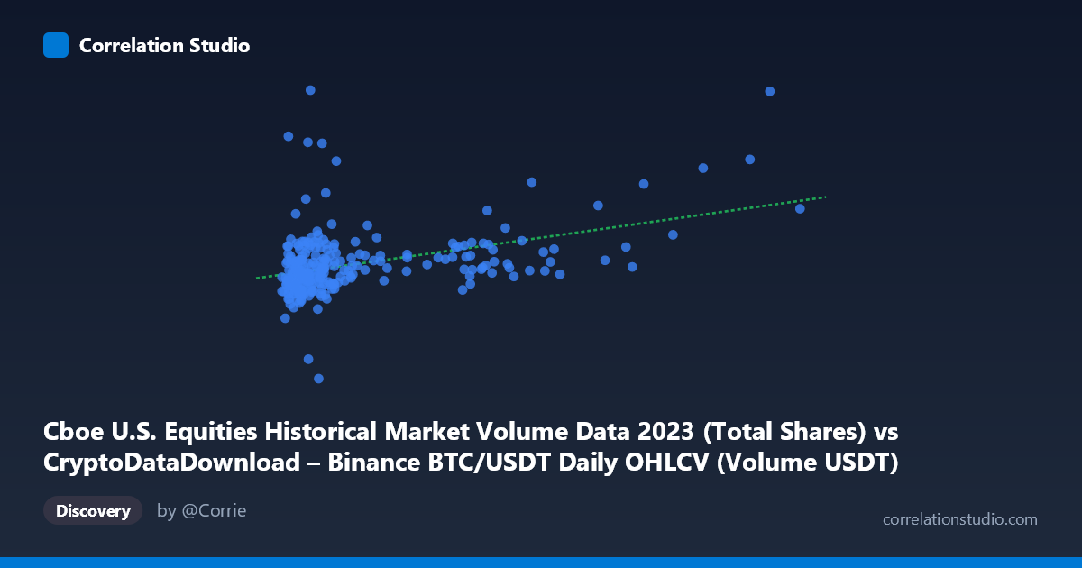
Cboe U.S. Equities Historical Market Volume Data 2023 (Total Shares) vs CryptoDataDownload – Binance BTC/USDT Daily OHLCV (Volume USDT)
- Pearson correlation (r)
- 0.4107
- Spearman correlation
- 0.415
- p-value
- 0
- Sample size (n)
- 250
- 95% confidence interval
- 0.302 to 0.5088
- Granger causality
- None
- Granger optimal lag
- 10
AI analysis
Analysis of Cboe U.S. Equities Volume vs. Binance BTC/USDT Volume (2023)
1. Relationship Overview
The scatterplot shows a weak-to-moderate positive relationship between two variables that appear to be mislabeled in the metadata (the X-axis is described as Cboe equities volume but contains BTC/USDT-scale values in the billions, while Y-axis values in the hundreds of millions align with equity volume figures). Regardless of labeling, the data shows most points clustered tightly in the lower-left region (X < 2 billion, Y between 450–650 million), with a long right tail of X values extending out to 17 billion. This heavy right-skew in X (mean 2.86B vs. median-like cluster around 1B, stdev 3.13B) indicates the distribution is far from normal, dominated by a handful of high-volume days.
2. Correlation Strength and Statistical Confidence
The Pearson correlation of r = 0.41 indicates a modest positive linear association, with r² = 0.169 meaning only ~17% of the variance in Y is explained by X — the remaining 83% is driven by other factors. The 95% CI [0.302, 0.509] is reasonably tight given n=250, and the p-value (1.37×10⁻¹¹) confirms the correlation is highly statistically significant — this is not due to chance, but statistical significance should not be conflated with practical strength or causal linkage. Critically, the Granger causality tests show no significant predictive direction in either direction (X→Y p=0.53; Y→X p=0.66), even at an optimal lag of 10 periods. This strongly suggests the contemporaneous correlation is not driven by one series temporally leading the other — instead it may reflect a shared external driver (e.g., overall market risk sentiment, macro volatility, or trading calendar effects) rather than a lead-lag trading relationship.
3. Notable Patterns and Outliers
Several high-leverage outliers are visible: points like (13.3B, 662M), (17.47B, max X), and (8.6B, 563M) sit far right of the main cloud and likely have outsized influence on the regression slope (0.012) and correlation coefficient — a Cook's distance or leverage check is warranted. There's also a low-Y outlier at (1.69B, 265.5M) — the minimum Y value — and a high-Y outlier at (695M, 933M), the maximum Y value, both of which deviate from the main trend and could reflect anomalous single-day events (e.g., a market holiday, flash crash, or data error). The bulk of the relationship (excluding the tail) appears nearly flat/noisy, suggesting the "trend" is substantially propped up by the handful of extreme-X points rather than a consistent linear pattern throughout the range.
4. Confounding Factors and Caveats
Several caveats apply: (1) Heteroscedasticity — variance in Y does not appear constant across X, violating a key linear regression assumption; (2) Non-normality/skew in X suggests a log transformation of X (and possibly Y) would better reveal the true relationship and reduce leverage from extreme values; (3) Both series are daily time-series data over one year, meaning autocorrelation within each series (common in volume data due to weekly/monthly cycles) could inflate the apparent cross-correlation without genuine dependency; (4) Shared macro confounders — both crypto and equity markets can react to the same news events (Fed announcements, CPI releases, risk-off days) — creating spurious correlation without any causal link between the specific exchanges' volumes.
5. Suggestions for Further Investigation
- Log-transform X (given its 3+ orders of magnitude range) and re-run correlation/regression to check if the relationship is more linear in log-space, and to reduce outlier leverage. - Remove or separately analyze the top 5-10 extreme X outliers to test whether the r=0.41 correlation holds in the "typical" data range or is an artifact of a few extreme days. - Test for common confounders: incorporate a market volatility index (e.g., VIX, BTC realized volatility) as a control variable to see if it explains the shared movement better than a direct X-Y link. - Given the null Granger causality result, do not use one series to forecast the other; if predictive modeling is the goal, look for other explanatory variables or consider this pair as parallel-but-independent time series. - Investigate the specific dates behind the outlier points (especially the 265M Y-value and 17.47B X-value) to determine if they reflect genuine market events or data quality issues.
X dataset: CryptoDataDownload – Binance BTC/USDT Daily OHLCV
Y dataset: Cboe U.S. Equities Historical Market Volume Data 2023
Part of experiment: Bitcoin - CryptoDataDownload – Binance BTC/USDT Daily OHLCV vs Cboe U.S. Equities Historical Market Volume Data 2023