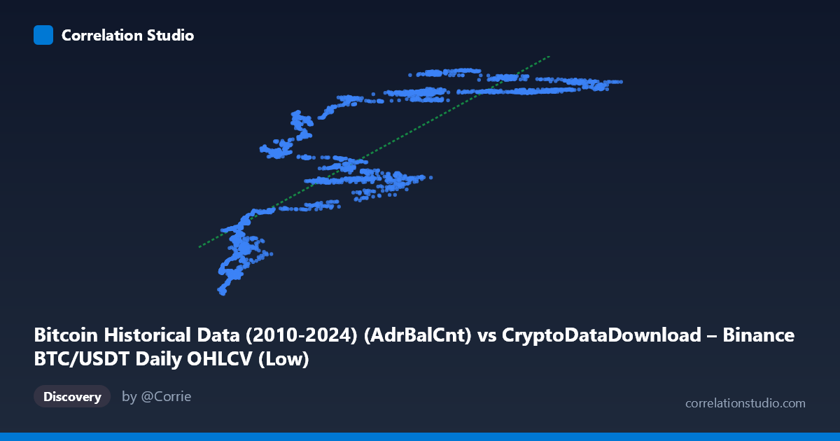
Bitcoin Historical Data (2010-2024) (AdrBalCnt) vs CryptoDataDownload – Binance BTC/USDT Daily OHLCV (Low)
- Pearson correlation (r)
- 0.8293
- Spearman correlation
- 0.9003
- p-value
- 0
- Sample size (n)
- 3191
- 95% confidence interval
- 0.8181 to 0.8398
- Granger causality
- None
- Granger optimal lag
- 10
- Time coverage
- 2017-08-17 to 2026-05-20
AI analysis
Analysis: Bitcoin Active Address Count vs. Daily Low Price
1. Overall Relationship
The scatterplot shows a strong positive association between Bitcoin's Active Address Count (X) and the daily Low price (Y). As network activity (unique addresses transacting) increases, the price tends to rise as well, though the relationship is not perfectly linear — it appears to flatten and show more dispersion at higher address counts, suggesting diminishing marginal price sensitivity to address growth once activity is already elevated.
2. Strength, Direction, and Predictive Direction
With r = 0.829 and r² = 0.688, roughly 69% of the variance in Bitcoin's price low is statistically associated with variance in active address count — a strong but not deterministic relationship. The remaining ~31% is driven by other factors (macro sentiment, liquidity, regulatory news, derivatives markets, etc.). The 95% CI [0.818, 0.840] is tight given the large sample (n=3,191), and the p-value of ~0 confirms this correlation is highly unlikely to be due to chance. However, the Granger causality results are the most important caveat: neither direction shows significant predictive power at conventional thresholds (X→Y: p=0.150; Y→X: p=0.054, only marginally short of significance). This means that despite the strong contemporaneous correlation, neither series reliably "leads" the other in a forecasting sense — address activity does not clearly predict future price moves, nor vice versa. This is a classic case where correlation does not imply temporal causation; both variables likely respond to shared underlying drivers (adoption cycles, bull/bear market phases) rather than one mechanically driving the other.
3. Patterns, Clusters, and Non-linearity
The sample points reveal a two-cluster structure: a low-X/low-Y cluster (X < 15,000, Y ~19M–33M) representing bear-market/early periods, and a high-X/high-Y cluster (X 55,000, Y ~50M–57M) representing bull-market periods with high network usage and elevated prices. There's a visible gap/transition zone (X ≈ 20,000–50,000) where Y values are more variable (ranging 33M–52M) — points like (23,433, 33.3M) and (57,071, 37.2M) show that similar address counts can correspond to quite different price levels, indicating regime-dependent behavior rather than a stable linear function. This is consistent with power-law or logistic-type relationships often seen in network-value models (e.g., Metcalfe's Law variants), where the linear fit (slope ≈ 310.7, intercept ≈ 27.7M) is a reasonable approximation but likely understates curvature.
4. Confounding Factors and Caveats
Several confounds warrant caution: - Time-trend confounding: Both series likely trend upward over the 2017–2026 window due to secular BTC adoption and price appreciation, inflating correlation without implying direct mechanistic linkage (spurious trend correlation). - Non-stationarity: Price and address counts are both non-stationary time series; standard correlation/regression on non-stationary data can overstate relationships (cointegration testing would be more appropriate). - Market regime effects: Bull/bear cycles (visible in the clustering) mean the relationship may hold differently across regimes — a single global r may mask regime-specific dynamics. - Exchange-specific bias: Data sourced solely from Binance OHLCV; on-chain address counts are network-wide, so exchange-specific volume/liquidity shocks (e.g., listing events, wash trading) could inject noise unrelated to genuine network growth.
5. Suggested Next Steps
- Test for cointegration (e.g., Engle-Granger or Johansen) rather than relying on simple correlation, given the non-stationary, trending nature of both series. - Segment analysis by market regime (bull vs. bear, or by year) to see if the r² and slope are stable or regime-dependent. - Detrend or difference both series (e.g., % change in addresses vs. % change in price) and re-run correlation/Granger tests to isolate short-term co-movement from shared long-term trend. - Given the marginal Y→X Granger result (p=0.054), it may be worth extending the lag structure or sample period to check if price modestly leads on-chain activity (e.g., speculative price rallies attracting new users) — a plausible behavioral hypothesis worth formal testing.
X dataset: CryptoDataDownload – Binance BTC/USDT Daily OHLCV
Y dataset: Bitcoin Historical Data (2010-2024)
Part of experiment: Bitcoin - CryptoDataDownload – Binance BTC/USDT Daily OHLCV vs Bitcoin Historical Data (2010-2024)