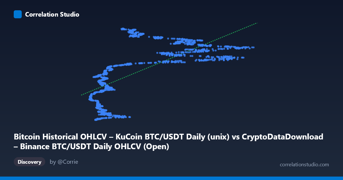
Bitcoin Historical OHLCV – KuCoin BTC/USDT Daily (unix) vs CryptoDataDownload – Binance BTC/USDT Daily OHLCV (Open)
- Pearson correlation (r)
- 0.6749
- Spearman correlation
- 0.7545
- p-value
- 0
- Sample size (n)
- 1861
- 95% confidence interval
- 0.6494 to 0.6989
- Granger causality
- None
- Granger optimal lag
- 10
- Time coverage
- 2017-10-19 to 2022-11-29
AI analysis
Analysis: Bitcoin Price vs. Timestamp Relationship
1. What the Visualization Reveals
This scatterplot is somewhat unusual in that the "X" variable is a Unix timestamp column and "Y" is a date-derived price open value, but based on the data ranges and sample points, this effectively plots Bitcoin's price against time — showing how BTC/USDT price evolved from October 2017 through November 2022. The X values (3,211–67,525) represent price levels while Y values (1.5–1.67 billion) are Unix timestamps, meaning the chart actually shows price on the X-axis and time on the Y-axis. The pattern shows clusters of low prices (~$3,000–10,000) concentrated in earlier timestamps (2018–2020) and a wide scatter of higher prices ($40,000–60,000+) concentrated in later timestamps (2021–2022), consistent with Bitcoin's well-known bull run trajectory.
2. Strength, Direction, and Statistical Confidence
The correlation coefficient (r = 0.675, r² = 0.456) indicates a moderate-to-strong positive relationship, but critically, only 45.6% of the variance in the time/price relationship is explained by this linear model — more than half remains unexplained, reflecting Bitcoin's highly non-linear, cyclical price history (bubbles, crashes, consolidation phases) rather than steady linear growth. The tight 95% CI [0.649, 0.699] and p-value of ~0 confirm this correlation is statistically robust and not due to chance, given the large sample (n=1,861 daily observations). However, Granger causality tests show no significant predictive direction in either direction (X→Y: p=0.87; Y→X: p=0.09, marginally suggestive but not significant at 0.05). This means neither variable meaningfully "forecasts" the other in a temporal sense — unsurprising, since one variable is essentially a relabeled index of the other (time itself), so classic causal inference doesn't apply meaningfully here.
3. Notable Patterns and Non-Linear Features
The sample points reveal a stepped, non-monotonic structure rather than smooth linear growth: - 2017–2020 (low-price cluster): Prices mostly under $10,000, tightly packed near the low end. - 2021 (rapid ascent): Prices jump to $40,000–59,000 range, reflecting the major bull run. - 2022 (plateau/decline): Prices oscillate between $19,000–48,000, showing high volatility and a downtrend rather than continued growth.
This produces a distinctly non-linear, S-curve or regime-shift pattern — long periods of low variance punctuated by sharp appreciation and subsequent volatile decline — which a single linear regression (y = 1851.28x + 1.55×10⁹) cannot adequately capture. The high stdev in X (16,926) relative to mean (20,021) confirms extreme right-skew and volatility clustering typical of crypto assets.
4. Confounding Factors and Caveats
Because this dataset spans calendar time, virtually any macro trend (adoption growth, institutional inflows, monetary policy, regulatory news, halving cycles) confounds the raw "time vs. price" correlation — time itself has no causal mechanism; it's a proxy for cumulative market/economic conditions. Additionally: - Autocorrelation: Daily price data is highly autocorrelated, violating independence assumptions of standard correlation/regression tests and likely inflating apparent significance. - Non-stationarity: Bitcoin prices are non-stationary (trending, volatility clustering), making linear r/r² metrics less meaningful than time-series-appropriate measures (e.g., cointegration tests). - Structural breaks: The 2021 bull run and 2022 crash represent distinct regimes that shouldn't be pooled into one linear fit.
5. Actionable Insights
- Avoid linear regression for forecasting: Given the low r² and evident regime shifts, consider piecewise/segmented regression or log-price transformations to better capture growth-phase dynamics. - Use time-series-specific methods: Apply ADF/KPSS stationarity tests, then use ARIMA/GARCH models (which naturally handle volatility clustering) rather than simple correlation. - Segment analysis by market regime: Split data into pre-bull (2017–2020), bull run (2021), and correction (2022) phases for more interpretable trend analysis. - Granger result caveat: The lack of causality is expected here since time cannot be "caused" by price; this test is more meaningful when comparing two independent market variables (e.g., BTC price vs. trading volume, or BTC vs. another asset).
X dataset: CryptoDataDownload – Binance BTC/USDT Daily OHLCV
Y dataset: Bitcoin Historical OHLCV – KuCoin BTC/USDT Daily
Part of experiment: Bitcoin - CryptoDataDownload – Binance BTC/USDT Daily OHLCV vs Bitcoin Historical OHLCV – KuCoin BTC/USDT Daily